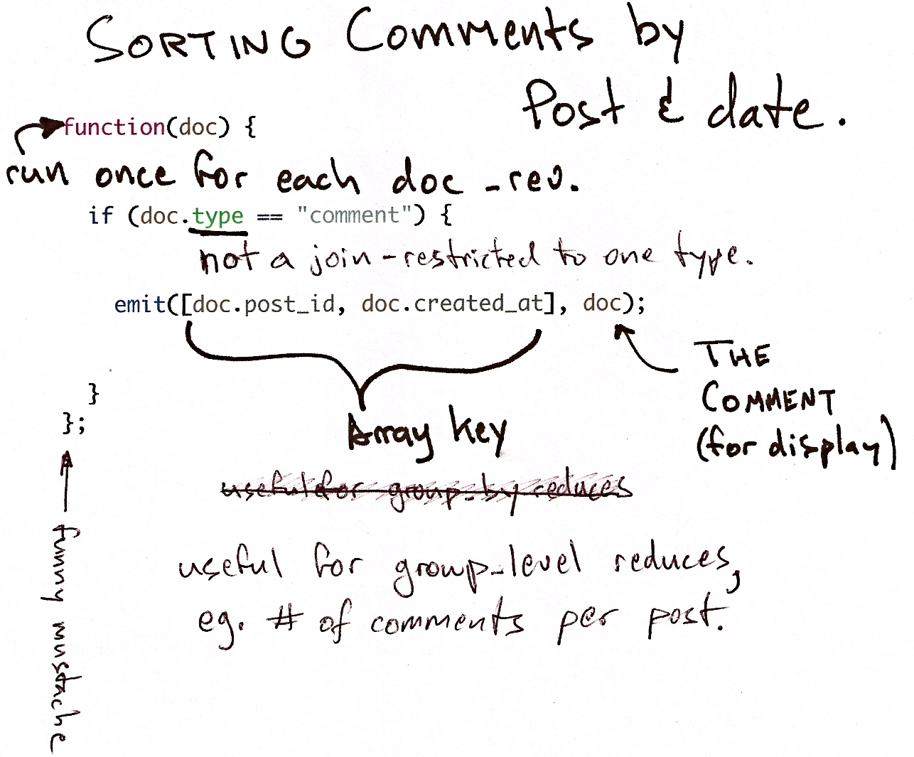
Figure 1. Comments map function
Views sind in verschiedenen Situationen nützlich:
Schauen wir uns die verschiedenen Szenarien etwas genauer an. Als erstes betrachten wir den Fall, indem Daten extrahiert und in eine bestimmte Reihenfolge gebracht werden müssen. Für eine Blogseite beispielsweise benötigen wir die Überschriften der Blog Postings sortiert nach Datum. Im Folgenden werden wir mit einigen Beispieldokumenten arbeinit, um zu zeigen wie Views funktionieren.
{
  "_id":"biking",
  "_rev":"AE19EBC7654",

  "title":"Biking",
  "body":"My biggest hobby is mountainbiking. The other day...",
  "date":"2009/01/30 18:04:11"
}

{
  "_id":"bought-a-cat",
  "_rev":"4A3BBEE711",

  "title":"Bought a Cat",
  "body":"I went to the the pet store earlier and brought home a little kitty...",
  "date":"2009/02/17 21:13:39"
}

{
  "_id":"hello-world",
  "_rev":"43FBA4E7AB",

  "title":"Hello World",
  "body":"Well hello and welcome to my new blog...",
  "date":"2009/01/15 15:52:20"
}
Drei reichen für das Beispiel aus. Achten sie darauf, dass die Dokumente nach "_id" sortiert sind - so wie sie auch in der Datenbank gespeichert sind. Nun legen wir eine View an. In Kapitel 3: Der Anfang wurde gezeigt, wie man eine View in Futon, dem CouchDB Admin UI anlegt. Fangen wir zunächst mit etwas Code an:
function(doc) {
  if(doc.date && doc.title) {
    emit(doc.date, doc.title);
  }
}
Das ist eine Map Funktion, die in JavaScript geschrieben ist. Falls sie wenig oder keine Erfahrung mit JavaScript, dafür aber mit C oder C-ähnlichen Sprachen wie Java, PHP oder C# haben, sollte das vertraut aussehen. Es ist eine einfache Funktionsdefintion.
Views werden in CouchDB als Strings im views Attribut eines Design Dokuments gespeichert. Man führt sie nicht selber aus, sondern wenn man die View abfragt, liest CouchDB den Source Code und führt ihn für jedes Dokument in der Datenbank, in der die View angelegt wurde, aus. Durch das Abfragen der View erhält man die View Ergebnismenge.
Alle Map Funktionen haben nur einen Parameter doc. Er enthält ein einzelnes Dokument der Datenbank. Unsere Map Funktion prüft, ob das Dokument ein date und ein title Attribut besitzt, was bei all unseren Dokumenten der Fall ist. Anschließend ruft die Map Funktion die eingebaute emit() Funtion mit diesen beiden Attributen als Argumenten auf.
Die emit() Funktion erwartet immer zwei Argumente: Zunächst den key (Schlüssel) und anschließend den value (Wert). Die emit(key,value) Funktion erzeugt einen Eintrag in der View Ergebnismenge. Man kann die emit() Funktion auch mehrfach in einer Map Funktion aufrufen, um mehrere Einträge in der Ergebnismenge zu erzeugen, doch darauf kommen wir später noch zurück.
CouchDB nimmt jeden Wert, den man der emit() Funktion übergibt und speichert ihn in einer Liste (siehe auch Tabelle 1: “View Ergebnismenge”). Jede Zeile in dieser Liste enthält einen Schlüssel und einen Wert. Was noch wichtiger ist: die Liste ist nach dem Schlüssel aufsteigend sortiert (in unserem Fall doc.date). Das ist die wichtigste Eigenschaft einer View. Ihr Ergebnis ist nach dem Schlüssel sortiert. Darauf werden wir immer wieder zurückkommen um noch andere nette Dinge zu tun.
| Key | Value |
|---|---|
"2009/01/15 15:52:20" | "Hello World" |
"2009/01/30 18:04:11" | "Biking" |
"2009/02/17 21:13:39" | "Bought a Cat" |
Tabelle 1: View Ergebnismenge
If you read carefully over the last few paragraphs, one part stands out: “When you query your view, CouchDB takes the source code and runs it for you on every document in the database.” If you have a lot of documents, that takes quite a bit of time and you might wonder if it is not horribly inefficient to do this. Yes, it would be, but CouchDB is designed to avoid any extra costs: it only runs through all documents once, when you first query your view. If a document is changed, the map function is only run once, to recompute the keys and values for that single document.
The view result is stored in a B-tree, just like the structure that is responsible for holding your documents. View B-trees are stored in their own file, so that for high-performance CouchDB usage, you can keep views on their own disk. The B-tree provides very fast lookups of rows by key, as well as efficient streaming of rows in a key range. In our example, a single view can answer all questions that involve time: “Give me all the blog posts from last week” or “last month” or “this year.” Pretty neat. Read more about how CouchDB’s B-trees work in Appendix F, The Power of B-trees.
When we query our view, we get back a list of all documents sorted by date. Each row also includes the post title so we can construct links to posts. Figure 1 is just a graphical representation of the view result. The actual result is JSON-encoded and contains a little more metadata:
{
  "total_rows": 3,
  "offset": 0,
  "rows": [
    {
      "key": "2009/01/15 15:52:20",
      "id": "hello-world",
      "value": "Hello World"
    },

    {
      "key": "2009/02/17 21:13:39",
      "id": "bought-a-cat",
      "value": "Bought a Cat"
    },

    {
      "key": "2009/01/30 18:04:11",
      "id": "biking",
      "value": "Biking"
    }
  ]
}
Now, the actual result is not as nicely formatted and doesn’t include any superfluous whitespace or newlines, but this is better for you (and us!) to read and understand. Where does that "id" member in the result rows come from? That wasn’t there before. That’s because we omitted it earlier to avoid confusion. CouchDB automatically includes the document ID of the document that created the entry in the view result. We’ll use this as well when constructing links to the blog post pages.
Let’s move on to the second use case for views: “building efficient indexes to find documents by any value or structure that resides in them.” We already explained the efficient indexing, but we skipped a few details. This is a good time to finish this discussion as we are looking at map functions that are a little more complex.
First, back to the B-trees! We explained that the B-tree that backs the key-sorted view result is built only once, when you first query a view, and all subsequent queries will just read the B-tree instead of executing the map function for all documents again. What happens, though, when you change a document, add a new one, or delete one? Easy: CouchDB is smart enough to find the rows in the view result that were created by a specific document. It marks them invalid so that they no longer show up in view results. If the document was deleted, we’re good—the resulting B-tree reflects the state of the database. If a document got updated, the new document is run through the map function and the resulting new lines are inserted into the B-tree at the correct spots. New documents are handled in the same way. Appendix F, The Power of B-trees demonstrates that a B-tree is a very efficient data structure for our needs, and the crash-only design of CouchDB databases is carried over to the view indexes as well.
To add one more point to the efficiency discussion: usually multiple documents are updated between view queries. The mechanism explained in the previous paragraph gets applied to all changes in the database since the last time the view was queried in a batch operation, which makes things even faster and is generally a better use of your resources.
On to more complex map functions. We said “find documents by any value or structure that resides in them.” We already explained how to extract a value by which to sort a list of views (our date field). The same mechanism is used for fast lookups. The URI to query to get a view’s result is /database/_design/designdocname/_view/viewname. This gives you a list of all rows in the view. We have only three documents, so things are small, but with thousands of documents, this can get long. You can add view parameters to the URI to constrain the result set. Say we know the date of a blog post. To find a single document, we would use /blog/_design/docs/_view/by_date?key="2009/01/30 18:04:11" to get the “Biking” blog post. Remember that you can place whatever you like in the key parameter to the emit() function. Whatever you put in there, we can now use to look up exactly—and fast.
Note that in the case where multiple rows have the same key (perhaps we design a view where the key is the name of the post’s author), key queries can return more than one row.
We talked about “getting all posts for last month.” If it’s February now, this is as easy as /blog/_design/docs/_view/by_date?startkey="2010/01/01 00:00:00"&endkey="2010/02/00 00:00:00". The startkey and endkey parameters specify an inclusive range on which we can search.
To make things a little nicer and to prepare for a future example, we are going to change the format of our date field. Instead of a string, we are going to use an array, where individual members are part of a timestamp in decreasing significance. This sounds fancy, but it is rather easy. Instead of:
{
  "date": "2009/01/31 00:00:00"
}
we use:
"date": [2009, 1, 31, 0, 0, 0]
Our map function does not have to change for this, but our view result looks a little different. See Table 2, “New view results”.
| Key | Value |
|---|---|
[2009, 1, 15, 15, 52, 20] | "Hello World" |
[2009, 2, 17, 21, 13, 39] | "Biking" |
[2009, 1, 30, 18, 4, 11] | "Bought a Cat" |
Table 2. New view results
And our queries change to /blog/_design/docs/_view/by_date?key=[2009, 1, 1, 0, 0, 0] and /blog/_design/docs/_view/by_date?key=[2009, 01, 31, 0, 0, 0]. For all you care, this is just a change in syntax, not meaning. But it shows you the power of views. Not only can you construct an index with scalar values like strings and integers, you can also use JSON structures as keys for your views. Say we tag our documents with a list of tags and want to see all tags, but we don’t care for documents that have not been tagged.
{
  ...
  tags: ["cool", "freak", "plankton"],
  ...
}
{
  ...
  tags: [],
  ...
}
function(doc) {
  if(doc.tags.length > 0) {
    for(var idx in doc.tags) {
      emit(doc.tags[idx], null);
    }
  }
}
This shows a few new things. You can have conditions on structure (if(doc.tags.length > 0)) instead of just values. This is also an example of how a map function calls emit() multiple times per document. And finally, you can pass null instead of a value to the value parameter. The same is true for the key parameter. We’ll see in a bit how that is useful.
To retrieve view results in reverse order, use the descending=true query parameter. If you are using a startkey parameter, you will find that CouchDB returns different rows or no rows at all. What’s up with that?
It’s pretty easy to understand when you see how view query options work under the hood. A view is stored in a tree structure for fast lookups. Whenever you query a view, this is how CouchDB operates:
startkey specifies, if present.endkey, if present.If you specify descending=true, the reading direction is reversed, not the sort order of the rows in the view. In addition, the same two-step procedure is followed.
Say you have a view result that looks like this:
| Key | Value |
|---|---|
0 | "foo" |
1 | "bar" |
2 | "baz" |
Here are potential query options: ?startkey=1&descending=true. What will CouchDB do? See #1 above: it jumps to startkey, which is the row with the key 1, and starts reading backward until it hits the end of the view. So the particular result would be:
| Key | Value |
|---|---|
1 | "bar" |
0 | "foo" |
This is very likely not what you want. To get the rows with the indexes 1 and 2 in reverse order, you need to switch the startkey to endkey: endkey=1&descending=true:
| Key | Value |
|---|---|
2 | "baz" |
1 | "bar" |
Now that looks a lot better. CouchDB started reading at the bottom of the view and went backward until it hit endkey.
We use an array key here to support the group_level reduce query parameter. CouchDB’s views are stored in the B-tree file structure (which will be described in more detail later on). Because of the way B-trees are structured, we can cache the intermediate reduce results in the non-leaf nodes of the tree, so reduce queries can be computed along arbitrary key ranges in logarithmic time. See Figure 1, “Comments map function”.
In the blog app, we use group_level reduce queries to compute the count of comments both on a per-post and total basis, achieved by querying the same view index with different methods. With some array keys, and assuming each key has the value 1:
["a","b","c"]
["a","b","e"]
["a","c","m"]
["b","a","c"]
["b","a","g"]
the reduce view:
function(keys, values, rereduce) {
  return sum(values)
}
returns the total number of rows between the start and end key. So with startkey=["a","b"]&endkey=["b"] (which includes the first three of the above keys) the result would equal 3. The effect is to count rows. If you’d like to count rows without depending on the row value, you can switch on the rereduce parameter:
function(keys, values, rereduce) {
  if (rereduce) {
    return sum(values);
  } else {
    return values.length;
  }
}

Figure 1. Comments map function
This is the reduce view used by the example app to count comments, while utilizing the map to output the comments, which are more useful than just 1 over and over. It pays to spend some time playing around with map and reduce functions. Futon is OK for this, but it doesn’t give full access to all the query parameters. Writing your own test code for views in your language of choice is a great way to explore the nuances and capabilities of CouchDB’s incremental MapReduce system.
Anyway, with a group_level query, you’re basically running a series of reduce range queries: one for each group that shows up at the level you query. Let’s reprint the key list from earlier, grouped at level 1:
["a"]   3
["b"]   2
And at group_level=2:
["a","b"]   2
["a","c"]   1
["b","a"]   2
Using the parameter group=true makes it behave as though it were group_level=Exact, so in the case of our current example, it would give the number 1 for each key, as there are no exactly duplicated keys.
We briefly talked about the rereduce parameter to your reduce function. We’ll explain what’s up with it in this section. By now, you should have learned that your view result is stored in B-tree index structure for efficiency. The existence and use of the rereduce parameter is tightly coupled to how the B-tree index works.
Consider the map result shown in Example 1, “Example view result (mmm, food)”.
"afrikan", 1
"afrikan", 1
"chinese", 1
"chinese", 1
"chinese", 1
"chinese", 1
"french", 1
"italian", 1
"italian", 1
"spanish", 1
"vietnamese", 1
"vietnamese", 1
Example 1. Example view result (mmm, food)
When we want to find out how many dishes there are per origin, we can reuse the simple reduce function shown earlier:
function(keys, values, rereduce) {
  return sum(values);
}
Figure 2, “The B-tree index” shows a simplified version of what the B-tree index looks like. We abbreviated the key strings.
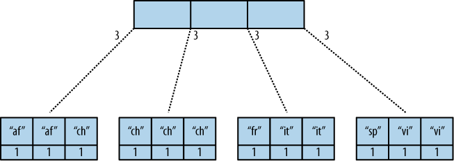
Figure 2. The B-tree index
The view result is what computer science grads call a “pre-order” walk through the tree. We look at each element in each node starting from the left. Whenever we see that there is a subnode to descend into, we descend and start reading the elements in that subnode. When we have walked through the entire tree, we’re done.
You can see that CouchDB stores both keys and values inside each leaf node. In our case, it is simply always 1, but you might have a value where you count other results and then all rows have a different value. What’s important is that CouchDB runs all elements that are within a node into the reduce function (setting the rereduce parameter to false) and stores the result inside the parent node along with the edge to the subnode. In our case, each edge has a 3 representing the reduce value for the node it points to.
In reality, nodes have more than 1,600 elements in them. CouchDB computes the result for all the elements in multiple iterations over the elements in a single node, not all at once (which would be disastrous for memory consumption).
Now let’s see what happens when we run a query. We want to know how many "chinese" entries we have. The query option is simple: ?key="chinese". See Figure 3, “The B-tree index reduce result”.
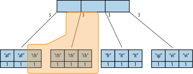
Figure 3. The B-tree index reduce result
CouchDB detects that all values in the subnode include the "chinese" key. It concludes that it can take just the 3 value associated with that node to compute the final result. It then finds the node left to it and sees that it’s a node with keys outside the requested range (key= requests a range where the beginning and the end are the same value). It concludes that it has to use the "chinese" element’s value and the other node’s value and run them through the reduce function with the rereduce parameter set to true.
The reduce function effectively calculates 3 + 1 on query time and returns the desired result. Example 2, “The result is 4” shows some pseudocode that shows the last invocation of the reduce function with actual values.
function(null, [3, 1], true) {
  return sum([3, 1]);
}
Example 2. The result is 4
Now, we said your reduce function must actually reduce your values. If you see the B-tree, it should become obvious what happens when you don’t reduce your values. Consider the following map result and reduce function. This time we want to get a list of all the unique labels in our view:
"abc", "afrikan"
"cef", "afrikan"
"fhi", "chinese"
"hkl", "chinese"
"ino", "chinese"
"lqr", "chinese"
"mtu", "french"
"owx", "italian"
"qza", "italian"
"tdx", "spanish"
"xfg", "vietnamese"
"zul", "vietnamese"
We don’t care for the key here and only list all the labels we have. Our reduce function removes duplicates; see Example 3, “Don’t use this, it’s an example broken on purpose”.
function(keys, values, rereduce) {
  var unique_labels = {};
  values.forEach(function(label) {
    if(!unique_labels[label]) {
      unique_labels[label] = true;
    }
  });

  return unique_labels;
}
Example 3. Don’t use this, it’s an example broken on purpose
This translates to Figure 4, “An overflowing reduce index”.
We hope you get the picture. The way the B-tree storage works means that if you don’t actually reduce your data in the reduce function, you end up having CouchDB copy huge amounts of data around that grow linearly, if not faster with the number of rows in your view.
CouchDB will be able to compute the final result, but only for views with a few rows. Anything larger will experience a ridiculously slow view build time. To help with that, CouchDB since version 0.10.0 will throw an error if your reduce function does not reduce its input values.
See Chapter 21, View Cookbook for SQL Jockeys for an example of how to compute unique lists with views.
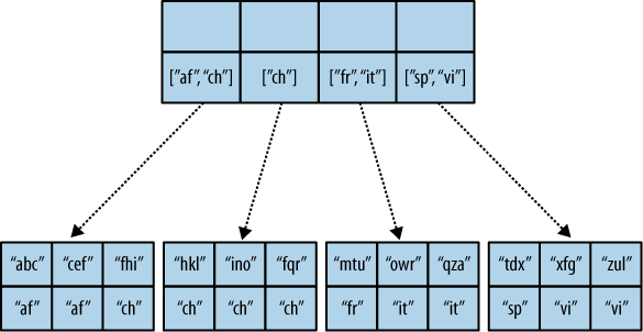
Figure 4. An overflowing reduce index
Map functions are side effect–free functions that take a document as argument and emit key/value pairs. CouchDB stores the emitted rows by constructing a sorted B-tree index, so row lookups by key, as well as streaming operations across a range of rows, can be accomplished in a small memory and processing footprint, while writes avoid seeks. Generating a view takes O(N), where N is the total number of rows in the view. However, querying a view is very quick, as the B-tree remains shallow even when it contains many, many keys.
Reduce functions operate on the sorted rows emitted by map view functions. CouchDB’s reduce functionality takes advantage of one of the fundamental properties of B-tree indexes: for every leaf node (a sorted row), there is a chain of internal nodes reaching back to the root. Each leaf node in the B-tree carries a few rows (on the order of tens, depending on row size), and each internal node may link to a few leaf nodes or other internal nodes.
The reduce function is run on every node in the tree in order to calculate the final reduce value. The end result is a reduce function that can be incrementally updated upon changes to the map function, while recalculating the reduction values for a minimum number of nodes. The initial reduction is calculated once per each node (inner and leaf) in the tree.
When run on leaf nodes (which contain actual map rows), the reduce function’s third parameter, rereduce, is false. The arguments in this case are the keys and values as output by the map function. The function has a single returned reduction value, which is stored on the inner node that a working set of leaf nodes have in common, and is used as a cache in future reduce calculations.
When the reduce function is run on inner nodes, the rereduce flag is true. This allows the function to account for the fact that it will be receiving its own prior output. When rereduce is true, the values passed to the function are intermediate reduction values as cached from previous calculations. When the tree is more than two levels deep, the rereduce phase is repeated, consuming chunks of the previous level’s output until the final reduce value is calculated at the root node.
A common mistake new CouchDB users make is attempting to construct complex aggregate values with a reduce function. Full reductions should result in a scalar value, like 5, and not, for instance, a JSON hash with a set of unique keys and the count of each. The problem with this approach is that you’ll end up with a very large final value. The number of unique keys can be nearly as large as the number of total keys, even for a large set. It is fine to combine a few scalar calculations into one reduce function; for instance, to find the total, average, and standard deviation of a set of numbers in a single function.
If you’re interested in pushing the edge of CouchDB’s incremental reduce functionality, have a look at Google’s paper on Sawzall, which gives examples of some of the more exotic reductions that can be accomplished in a system with similar constraints.